Stimulus determinants of the phenomenon of change blindness

Gusev, A.N. Lomonosov Moscow State University, Moscow, Russia

Mikhailova, O.A. Lomonosov Moscow State University, Moscow, Russia

Utochkin, I.S. National Research University "Higher School of Economics", Moscow, Russia

Change blindness is defined as the persistent inability to notice changes in a perceived scene because of a short disruption in perception (Falikman, 2006; Rensink, O’Regan, & Clark, 1997; Utochkin, 2011). Research of spatial attention with the use of change-detection tasks (involving “global disruption”) has been developing for over 40 years, starting with George McConkie’s research in the 1970s (Falikman, 2006). The most common experiments are those in which image changes are presented during saccadic eye movements or which involve an image shift or flickering. The flicker paradigm was introduced by Rensink et al. (1997). Two images (the original one and an altered one) are repeatedly alternated with a gray background; this procedure creates the special effect of flickering images. This type of image presentation doesn’t allow the observer to automatically notice even major changes. In the case of uninterrupted perception, any local change in the object is automatically registered by movement detectors and attracts involuntary attention. However, global disruption masks this local change, and the observer can’t pay attention to the changes automatically. Research shows that when a blank screen is presented between the original and the altered images, perception deteriorates. It becomes increasingly difficult to notice the changes even when they’re significant, repeated, and expected (Rensink et al., 1997; Simons & Chabris, 1999).

Simons and Levin(1998)deliberately included goofs[1] in short videos and found that observers experienced change blindness while watching them: they never noticed important changes, like a change in the lead actor. Even professional editors, despite their huge experience in working with video material, weren’t able to detect significant errors in the montage. Change blindness is particularly evident when the observer is not expecting any changes. In this case many observers are not able to notice that the man they had been talking to was secretly exchanged with another person. This research indicates that change blindness occurs because of different distractions, such as flickering, random noise, or flashes.

Modern scientists who study change blindness usually use different materials and traditionally present complex visual scenes to the observers (Gusev, Mikhailova, & Utochkin, 2012; Rensink et al., 1997; Simons & Levin, 1998; Utochkin, 2011). Only a small number of studies are based on simple stimuli (Goddard & Clifford, 2013; Irwin & Andrews, 1996).

Hypotheses

The first hypothesis of this study is that the intensity of change blindness depends on the physical characteristics of a visual pattern such as the number and location of objects (simple figures) within the pattern, their shape, distractions or the absence of distractions, and the interstimulus interval.

The second hypothesis is that the intensity of change blindness depends on the type of changes that occur within the image (appearance or disappearance of objects, change of color, or shifted location in the stimulus space).

Methods

Subjects (Observers)

Seventy-eight people aged 14 to 35 (average age, 21) with normal (or corrected-tonormal) vision participated in the empirical part of this study.

Stimuli and equipment

For the study of change blindness we created special stimulus material that allowed us to trace the connection of change blindness with memory and attention. The stimulus patterns consisted of several simple shapes — squares, triangles, circles, stars, diamonds, or their combinations (see Table 1). The shapes had either regular organization (structured images) or random organization (unstructured images). Four stimuli (numbers 1, 2, 5, and 6) each consisted of 5 simple shapes of different colors; 2 stimuli (3 and 4) each consisted of 20 shapes. In addition, the square shape was replaced with the word дом (house) in one of the stimuli. The size of a square shape on a 17-inch screen (as well as the maximum size of other shapes) was 0,0012 × 0,0012 m.

Table 1. Stimulus material

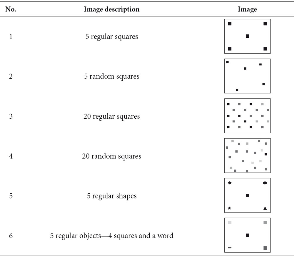
Note. Stimulus material can be found on the website of the UMK “Psychology” company: http:// psychosoft.ru.

The colors of the stimuli were chosen according to a standard 256-color palette. The stimuli with 5 squares had yellow, green, blue, brown, and red shapes. For the stimuli with 20 squares we used the same colors along with 15 extra colors (3 extras for each basic color) that were as close as possible in brightness to the original colors with equally different shades from the original.

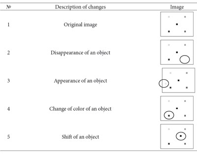
In order to study change blindness, many researchers use such types of change as appearance and disappearance or a location shift or color change in one of the objects (see Simons & Rensink, 2005a, 2005b). In this study we used all these types of changes.

Each stimulus had to undergo three types of changes—appearance/disappearance, change of color, and shift of an object (see Table 2). Each type of change had 5 variations: different trials included different objects within each stimulus. For appearance/disappearance, the following changes occurred in different trials: (1) disappearance of an object (2 variations); (2) appearance of an object (3 variations). The location of the appearance and the disappearance was controlled; it was closer to either the central or the peripheral area. Change of color was applied to 5 objects; each difference from the original in shades and altered objects was controlled and was labeled as “a slight difference,” “a medium difference,” or “a strong difference.” For shifting the location of 5 objects, we controlled their new location (central or peripheral) and the direction of change (toward or away from the center).

Table 2. Types of changes within stimulus material

In addition to trials with changes, some trials were run without changes (30% of the trials were without changes). The total number of sessions in this study was 120.

All types of sessions were randomized.

Using the flicker paradigm we made changes during the interstimulus interval, while a gray screen was being shown. Each trial cycle included successively a demonstration of the original image (400 ms), the interstimulus interval (200 ms), a demonstration of the altered image (400 ms), and the interstimulus interval (200 ms) (see Figure 1). Thus, each trial cycle lasted 1200 ms. In order to assess the influence of the interstimulus span we extended the interstimulus interval to 400 ms. The experimental plan was prepared and executed in a program called StimMake (by A. N. Gusev and A. E. Kremlev). The stimuli were demonstrated on a 17-inch PC screen and the whole screen was used for their presentation. The distance between the observer’s eyes and the screen was 0,6 m, approximately 54o. The cycle of stimuli demonstration within each trial was repeated until the observer stopped it by pressing one of the keys. Thus, the time for each trial and for the whole session was not limited. Observers’ answers and reaction times were recorded.

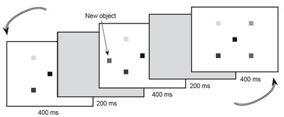
Figure 1. The cycle of successive image demonstrations in each trial

Procedure

Before the start of the session we informed each observer that he (she) was going to participate in an experiment related to visual attention and the task was to detect the element that changed in two successive demonstrations as soon as possible. The observer was to press the “left shift” key if he (she) detected a change and the “right shift” key if he (she) did not detect a change and to hold the key for 1 sec. As soon as the key was pressed, the trial cycle stopped and the original image appeared on the screen. After that the observer had to report the change that had been detected and point to its location.

Collected data were analyzed using the StimMake program, which allowed us to estimate the time of change detection for each trial and to assess the accuracy of the answers. Statistical analysis was performed in the IBM SPSS Statistic, version 19.0.

Results

Time of Change detection for different images

The results indicate that the easiest change for detection is appearance or disappearance of an object in a matrix with 5 regular shapes, while the most difficult change for detection is color in a matrix with 20 random shapes (see Table 3).

Table 3. Average time of change detection (number of cycles) and its dependence on the number of objects and their location

	Type of stimulus material	Average change-detection time, cycles
5	regular shapes	2.39
4	regular squares and a word	2.54
5	regular squares	2.61
5	random squares	2.66
5	regular squares, interstimulus interval 400 ms	3.11
20	regular squares	5.01
20	random squares	5.31

There were no statistically significant differences in time of average change detection between stimulus material with regular and random square shapes for the stimuli with both 5 (t(19) = 0.85, р = 0.41) and 20 (t(19) = 1.19, р=0.25) objects.

Change detection times for the stimuli with 5 and 20 squares for both regular (t(19) = 7.87, р<0.001) and random (t(19) = 7.46, р<0.001) organization were compared to examine statistical significance: increasing the number of shapes from 5 to 20 approximately doubled the increase in change-detection time (see Table 3).

Change-detection time was significantly lower for the stimuli with regular shapes compared with the stimuli that included only squares (t(19) = 3.34, р = 0.003).

Changing one of the squares to the word дом did not cause a significant increase in detection for any type of change (t(19) = 0.52, р = 0.61).

Increasing the interstimulus interval from 200 to 400 ms significantly increased the time of change detection by almost 20%. The difference was statistically significant (t(19) = 2.52, р = 0.02).

Thus, we can conclude that the most significant differences were found for the stimuli with 5 and 20 squares. Further analysis will focus on these particular stimuli.

Types of changes and their influence on time of change detection

The factor of image organization (regular or random squares) didn’t have any influence on change-detection time for the appearance/disappearance of objects and for a change in color. The results showed that the factor of image organization didn’t have any influence for the stimuli with 20 squares (appearance/disappearance: t(58)=–0.291, р=0.772; color change: t(37)=0.796, р=0.431) and for the stimuli with 5 squares (appearance/disappearance: t(58) = –1.337, р = 0.186; change of color: t(58)=0.297, р=0.767). However, there were statistically significant differences for this factor when 1 of the 20 objects was shifted (t(57) = 4.785, р<0.001) and quasi-significant differences when we shifted 1 out of 5 objects (t(58) = –1.781, р = 0.08).

Table 4. Average time of change detection in cycles (T) and percentage (%) of correct answers for different types of stimuli and different types of changes

Type of change		Appearance/disappearance		Color		Shift
Type of stimulus		T	%	T	%	T	%
5 squares	Regular	2.48	97.08	3.33	85.42	2.82	96.0
	Random	2.57	98.0	3.32	86.25	3.00	92.0
20 squares	Regular	4.50	80.67	6.64	38.33	4.47	80.0
	Random	4.41	76.0	6.97	37.0	5.57	67.0

In general, irrespective of the type of changes, the factor of image organization did not significantly affect change-detection time for images with 5 and 20 squares. The results of a 2-way ANOVA (analysis of variance) did not show any significant interaction between “organization” and “number of squares” (F = 2.819(1.37), р=0.102). Irrespective of the number of squares (5 or 20), there were no significant differences in change-detection time for both regular and random stimuli (t(37) = 1.660, р = 0.105; t(58) = –1.288, р = 0.203).

The time required for correct answers in trials with no changes was also analyzed. The results showed that change-detection time was longer for random objects compared with regular ones for stimuli with both 5 and 20 squares (t(59) = 3.165, р = 0.002; t(59) = 3.022, р = 0.004, respectively).

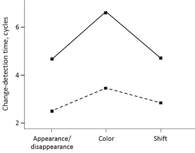
Figure 2. Dependence of the change-detection time on the number of squares and the types of change for stimuli with regular squares. The solid line shows stimuli with 20 squares; the dotted line shows stimuli with 5 squares.

Data for regular and random square shapes were analyzed separately. A 2-way ANOVA (Figure 2) demonstrated the high validity of the interaction effect for the following factors: “type of change” and “number of squares” (F = 7.585(2, 64.601), р = 0.003); we used the Greenhouse-Geisser correction while computing the F-statistic.

The most difficult task for change detection was change of color. Change-detection time for shifts was significantly shorter than for changing color for stimuli with both 5 and 20 squares (t(59) = 4.150, р<0.001; t(45) = –5.656, р<0.001 respectively).

The results for appearance/disappearance of squares were similar (t(58) = –6.359, р<0.001; t(45) = –5.860, р<0.001 respectively).

A comparison of change-detection time for appearance/disappearance and shifts showed significant differences for stimuli with 5 squares (t(58)=–4.445, р<0.001). However, the differences were not significant for stimuli with 20 squares (t(58) = 0.162, р = 0.872).

Furthermore, a highly valid dependence of the accuracy of answers on the number of squares and the type of stimuli changes with regular organization was found (see Figure 3): F = 33.025(2, 108.722), р<0.001; the Greenhouse-Geisser correction was used while computing the F-statistic.

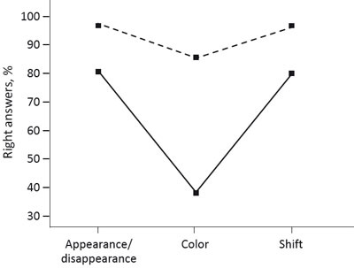
Figure 3. Dependence of the right answers (%) on the number of squares and the type of change for stimuli with regular organization. The solid line is for stimuli with 20 squares; the dotted line is for stimuli with 5 squares.

It is obvious that the most difficult task was the detection of color change. There were more correct answers for shifts than for color change for both 5 and 20 squares (t(59)=3.797, р<0.001; t(59)=11.383, р<0.001, respectively). Similar results were found for the appearance/disappearance of squares (t(59)=3.50, р = 0.001; t(59) = 11.684, р<0.001). There were no significant differences in correct answers for shifts and appearance/disappearance for either the 5 or the 20 squares (t(59) = –0.489, р = 0.627, t(59) = –0.244, р = 0.808, respectively).

Results of the interaction between the type of change and the number of squares for stimuli with random squares were similar (F=11.304(2, 71.912), р<0.001; the Greenhouse-Geisser correction was used for computing the F-statistic). Moreover, the parameters of the change-detection time for stimuli with 20 squares in the case of shifts and appearance/disappearance demonstrated statistically significant differences (t(58)=4.575, р<0.001).

The results for regular squares were similar. The analysis of correct answers has proved its dependence on two factors: the number of squares and the type of change (F=23.691(2, 102.525), р<0.001; the Greenhouse-Geisser correction was used for computing the F-statistic).

Color-change detection in 1 of 5 (or 20) squares with random images was compared with shifts (t(59)=-2.261, р=0.027; t(59)=-8.396, р<0.001, respectively) and appearance/disappearance (t(59)=-3;971, р<0;001; t(59)=-11;120, р<0;001, respectively). In contrast to regular shapes, the random ones showed significant differences for shifts and appearance/disappearance for both 5 and 20 squares (t(59)=2.735, р=0.008; t(59)=3.137, р=0.003, respectively).

Table 5. Effectiveness of visual detection for different degrees of color change

Type of color change	Image organization	Average time of detection, cycles	% of errors
Blue to yellow	Regular	2.31	0
Blue to yellow	Random	2.80	3
Green to red	Random	2.94	23
Red to brown	Regular	3.18	13
Red to yellow	Regular	3.22	10
Purple to red	Random	3.28	8
Green to blue	Regular	3.44	15
Brown to green	Regular	3.89	22
Green to yellow	Random	4.28	15
Green to red	Random	5.48	53
Black to light gray	Regular	5.91	45
Black to dark gray	Regular	6.14	55
Red to blue	Random	6.60	68
Pink to turquoise	Random	6.88	68
Orange to gray	Random	7.38	62
Turquoise to greenish-blue	Regular	7.41	68
Greenish-yellow to purple	Regular	7.58	57
Purple to yellow	Random	8.97	63
Orange to brown	Regular	10.34	80

Note. Lines are sorted according to increasing average time of change detection.

Changes occurring within the condition of color change varied and thus were examined separately. For example, stimuli with 20 regular or random squares were subject to 5 types of shading changes. The degree of shading change (e.g., from orange to brown or from red to green) influenced the effectiveness of change detection and its speed and accuracy (Table 5). In stimuli with 5 squares some of the color changes could be detected quicker and with greater accuracy (corresponding parameters were below average for this group of stimuli): blue to yellow and red to yellow. Color change for another group of stimuli (corresponding parameters were above average for this group of stimuli) was detected with greater difficulty: green to blue, brown to green, green to yellow.

A similar trend was observed among stimuli with 20 squares. We can select a group of stimuli in which color change was detected more effectively—green to red, black to light gray, red to blue—and a group in which change detection was less effective: orange to brown, purple to yellow, turquoise to greenish-blue, and orange to gray.

Discussion

Significant differences were found in the intensity of change blindness for different types of changes. In accordance with typical findings in cognitive psychology (Gegenfurtner & Sperling, 1993), Figure 4 demonstrates the distribution of stimuli as an operational characteristic of an average observer. It reflects the difficulty of a change-detection task on two dimensions, speed and accuracy. The results indicate that the intensity of this phenomenon depends on the conditions of detection, such as the number of objects, their organization, and the type of change. The most difficult condition for detection was color change within an image with many objects (C20RAN, C20REG), while the easiest was appearance/disappearance of an object in an image with a small number of objects (AD5REG, AD5RAN). Change detection of shifts (SH5RAN, SH5REG, SH20REG, SH20RAN) was in its complexity closer to appearance/disappearance detection than to change-of-color detection.

The number of objects in an image is another key factor affecting the degree of difficulty of a change-detection task. Similar effects were discovered in a study done by S. Luck and E. Vogel. Their study was based on similar stimulation and was focused on the analysis of color-change detection and its dependence on the number of square objects: increasing the number of colored squares from 4 to 12 decreased the percentage of correct answers from approximately 95% to 65% (Luck & Vogel, 1997). The main difference between their study and ours is that the accuracy of color-change detection in their study was much higher than the accuracy of detecting changes in location.

Regular organization of objects reduces the difficulty of change detection. This finding was especially explicit in the images with 20 squares. For example, AD20REG and SH20REG are located on the graph above the average level of correct change detection, while AD20RAN and SH20RAN are below.

Perhaps color change has no priority during processing because the changes occur within the object’s parameters, while appearance/disappearance and shifting change the object’s location and thus transform the whole visual scene.

Figure 4. Operational characteristic of the accomplishment of a change-detection task by an average observer. The Y axis shows the time of giving correct answers to a change-detection task; the X axis shows the probability of correct answers. Stimulation codes: AD — appearance/ disappearance of one of the squares, C — change of color, SH — shift, 5 and 20 — number of squares, REG — regular organization of shapes, RAN — random organization of shapes.

Perception of the location and color of objects by the human visual system is executed by channels consisting of different types of retinal ganglion cells (Muravyova, 2013). Retinal ganglion cells have been separated into two groups, magnocells and parvocells, according to their morphology and functions. The magnocellular system has optimal sensitivity to low-contrast and low-spatial frequency, and thus it can detect the direction of movement and can identify the parameters that are important for spatial orientation.

The distinguishing feature of the parvocellular system is its optimal sensitivity to high-contrast and high-spatial frequencies (Muravyova, 2013). This system provides color-change detection during visual analysis.

In order to prove the special role of color in the change-blindness phenomenon, irrespective of the number of shades that were subject to change in the stimuli with 20 squares (and thus separating the role of attention itself and the difficulty of discerning colors), we should pay special attention to the data received from stimuli with 5 squares. Although the factor of discerning difficulty has great importance, its influence on the stimuli with 5 squares is reduced.

Such cognitive processes as attention and memory are, undoubtedly, connected with change blindness (Hollingworth, Williams, & Henderson, 2001; O’Regan & Noë, 2001). In our opinion, the presence of a multitude of factors is evidence of a connection among memory, attention, and change-detection time. Further studies will focus on examination of this connection.

Acknowledgments

This work was supported in part by the Lomonosov Moscow State University Program of Development. The study was conducted with the financial support of the Ministry of Education and Science of the Russian Federation in the project “Development of methods for mapping and transfer of static and dynamic images, modeling of multimodal interfaces in immersive VR systems” (State contract 14.514.11.4035).

References

Alikman, M. V. (2006). Obshaya psichologiya [General psychology], Vol. 4: Attention. Moscow: Academy.

Gegenfurtner, K. R., & Sperling, G. (1993). Information transfer in iconic memory experiments. Journal of Experimental Psychology: Human Perception & Performance, 19(4), 845–866. doi: 10.1037/0096–1523.19.4.845

Goddard, E., & Clifford, C.W.G. (2013). A new type of change blindness: Smooth, isoluminant color changes are monitored on a coarse spatial scale. Journal of Vision, 13(5):20, 1–8.

Gusev, A., Mikhailova, O., & Utochkin, I. (2012). The role of individual differences in changeblindness. Voprosy Psikhologii [Issues in Psychology], 4, 117–128.

Hollingworth, A., Williams, C. C., & Henderson, J. M. (2001). Scene context and change blindness: Memory mediates change detection. Psychonomic Bulletin and Review, 8, 761–768.doi: 10.3758/BF03196215

Irwin, D. E., & Andrews, R. V. (1996). Integration and accumulation of information across saccadic eye movements. In T. Inui & J. L. McClelland (Eds.), Attention and performance XVI: Information integration in perception and communication(pp. 125–155). Cambridge, MA: MIT Press.

Levin, D.T., & Simons, D.J. (1997). Failure to detect changes to attended objects in motion pictures. Psychonomic Bulletin and Review 4(4): 501–506. doi: 10.3758/BF03214339

Luck, S. J., & Vogel, E. K. (1997). The capacity of visual working memory for features and conjunctions. Nature, 390, 279–281. doi: 10.1038/36846

Muravyova, S. V. (2013). Study of functional status of magnoand parvo-channel of human visual system. St. Petersburg: Abstract.

O’Regan, J. K., & Noё, A. (2001). A sensorimotor account of vision and visual consciousness. Behavioral and Brain Sciences, 24(5), 939–1031. doi: 10.1017/S0140525X01000115

Rensink, R. A., O’Regan, J. K., & Clark, J. J. (1997). To see or not to see: The need for attention to perceive changes in scenes. Psychological Science, 8, 368–373. doi: 10.1111/j.14679280.1997.tb00427.x

Rensink, R. A., O’Regan, J. K., & Clark, J. J. (2000). On the failure to detect changes in scenes across brief interruptions. Visual Cognition, 7(1/2/3), 127–145. doi: 10.1080/135062800394720

Simons, D. J., & Chabris, C. F. (1999). Gorillas in our midst: Sustained inattentional blindness for dynamic events. Perception, 28(9), 1059–1074. doi: 10.1068/p2952

Simons, D. J., & Levin, D. T. (1998). Failure to detect changes to people during a real-world interaction. Psychonomic Bulletin and Review, 5(4): 644–649. doi: 10.3758/BF03208840

Simons, D. J., & Rensink, R. A. (2005a). Change blindness: Past, present, and future. Trends in Cognitive Sciences, 9(1), 16–20. doi: 10.1016/j.tics.2004.11.006

Simons, D. J., & Rensink, R. A. (2005b). Change blindness, representations, and consciousness: Reply to Noё. Trends in Cognitive Sciences, 9(5), 219. doi: 10.1016/j.tics.2005.03.008

Utochkin, I. S. (2011). Hide-and-seek around the centre of interest: The dead zone of attention revealed by change blindness. Visual Cognition, 19(8), 1063–1088. doi: 10.1080/ 13506285.2011.613421

Notes

[1] Goofs are montage mistakes that connect to each other fragments of the shots of slightly different scenes. In the experiments of Levin and Simons (1997), they were made deliberately.